For questions, remarks, or suggestions please contact coreceptor@mpi-inf.mpg.de.
Several members of a new class of anti-HIV-1 drugs, trying to prevent the viral entry into the cell, have arrived at the final stage of the drug development pipeline. An important subclass of these entry inhibitors are drugs that target one of the receptors that can be used, in addition to the main receptor CD4, by HIV-1, as a coreceptor to enter the cell. The most important HIV coreceptors are the chemokine receptors CCR5 and CXCR4. HIV-1 particles fall into three classes according to which of them they can use to enter a cell: some can only use CCR5, others can only use CXCR4, and some can use either of them. Before and during drug treatment with a coreceptor antagonist it is important to find out about the coreceptor usage of the virus population in the patient. Currently, expensive and time-consuming experimental assays are used for this task. In contrast, bioinformatics methods for predicting coreceptor usage directly from the sequence are cheap and fast, because sequencing has become a routine task in biotechnology. geno2pheno[coreceptor] is such a bioinformatics tool, currently based on support vector machines: it predicts HIV-1 coreceptor usage from the V3 region of the HIV envelope protein gp120. It is very easy to use: you do not have to cut the V3 loop out of your sequences and you also don't have to align your sequence manually - geno2pheno[coreceptor] does all this automatically. The tool consists of two screens: when visiting the geno2pheno[coreceptor] web site, the input page is shown. Here you can paste in or upload your sequence, and adjust some options. On clicking the "align & predict" button, the output page will be displayed. This may take some seconds due to the computations that have to be performed.
The input page consists of five parts:
A field labeled "Identifier". Here you can type in supplementary information about the sequence. This is not obligatory, just an option that helps you not to confuse the printouts of the predictions: The identifier will be shown, along with other data, such as the FASTA header of the sequence (if available) and the date when the prediction has been made, as the first part of the output page.
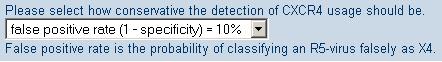
A box where you can select how conservative the predictions of CXCR4 usage will be. For example, if you adjust the CXCR4 classifier to be very conservative, only few sequences of viruses that cannot use CXCR4 will be predicted to be CXCR4-using. However, the drawback of a very conservative classifier is that there will be more CXCR4-using sequences which will remain undetected. This is the fundamental trade-off in classification. If, on the other hand, the classifier is adjusted not to be conservative, most sequences that can use CXCR4 will be detected, at the cost of a higher number of "false alarms, i.e. sequences for which CXCR4 usage is predicted by mistake. The technical details of how to adjust the degree of conservativeness will be explained below.
Two fields where you can input the sequence data. This can be done in two ways: The first way is to specify the name of a file to be uploaded. This can be done either by typing the file name directly into the upper of the two fields or by browsing for the file. The second way is to use the copy/paste mechanism of your web browser to paste the sequence data into the lower of the two fields. Whichever of the two ways you choose, your sequence data may either be in plain text or in FASTA-format. In case you want to have a batch run you save your sequences in a FASTA file and submit it to the webserver. The system will generate a prediction for each of these sequences and report them in a table that can be downloaded in csv-format (which can be opened with Excel, for instance). In this case you have to have to define the FPR cutoff by yourself. E.g. if you choose the standard cutoff of 10% then a value below 10% is predictive for an X4 virus whereas a value above 10% reflects an R5 virus. Further, it is no problem if, as a result of population sequencing, your sequence contains mixtures (non-unique nucleotides): our method can deal with them.
Additional clinical parameters.
The viral population in vivo is usually a mixture of heterogenous variants, often termed as the quasispecies.
To obtain a representative sample of this quasispecies, a substantial number of clones would have to be picked. However, in
routine clinical practice, this is not feasible. Instead, clinically derived samples are usually sequenced with population-
based or bulk approaches. In general, these techniques are unable to reliable detect minority species covering less than approximately
20% of the viral population. Furthermore, these sequences often contain mixtures of co-existing viruses which leads to a substantial
decrease in predictive performance in comparison to clonal data.
In a study on antiretroviral-naďve samples (Sing et al., 2007), it could be shown that additional clinical data
like CD4-cell counts can act as surrogate markers and improve predictive performance. The data in
this study has been used to train additional prediction models. By setting different clinical parameters, a second prediction
based on this additional information is displayed. However, it has to be emphasized
that these models are generated from antiretroviral-naďve samples.
The action box determining what is to be done. The most important option is labelled "align & predict". Upon selection this option, the V3 region will be extracted out of your sequence, an alignment will be computed, and a prediction will be made. The results will be shown on the output page, which is displayed when the computations are done. The "Reset form" option can be used to clear the form and to set the significance levels back to the default values. "Load a sample sequence" can be used to get to know the program without the need to supply a sequence. Finally, the "Switch to vertical layout" selection allows users with small displays to see the page properly.
As mentioned above, the significance levels let you adjust how conservative the prediction of CXCR4 usage will be. How to interpret it exactly is not difficult to understand and will be explained in this section.
Consider the picture above. Here, we have plotted a histogram of the scores for the tendency of the virus
to be X4-capable (can use CXCR4) that were predicted by our (old) method for sequences with known coreceptor usage. The plot was
computed for the task of detecting whether a virus is X4-capable. Thus the intention is that high scores indicate a high tendency
of the virus to be X4-capable and low scores indicate a tendency of the virus not to be X4-capable. In the plot, the x axis represents
the predicted scores, and the y axis shows the number of samples which were assigned a particular score by the method. The blue bars
represent the histogram of predicted values for the sequences that are not X4-capable, and the red bars show the histogram of
predicted values for those sequences that are X4-capable. Since the situation which is shown here is about detecting X4-capability,
those sequences that areX4-capable (shown in red) are called "positive" samples and those that are not are called "negative" samples.
The tendency that the positive samples attain a higher score than the negative samples is clearly visible from the plot above. However,
you can also see that there is significant overlap between the two distributions for the positive and negative samples, pespectively, so
perfect classification is not possible. This leaves us with the problem of how to choose an appropriate cutoff for prediction, such
that all samples that are assigned a score greater than the cutoff will be predicted as X4-capable and for all samples that are scored
below the cutoff, the prediction will be that the virus is not X4-capable. To understand the trade-off that arises, have a look at the
following picture, which is the same as above, but with three different possible cutoffs shown.
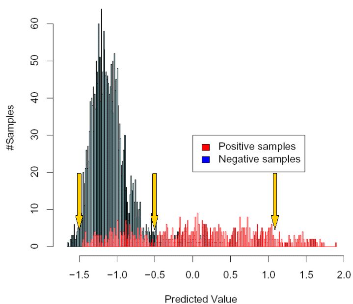
As a start, imagine that you select the leftmost of the three cutoffs that are shown,
at the value -1.5. This means that if a sample is scored below -1.5, the virus is predicted as not
X4-capable, and if it is scored above -1.5, the prediction is that the virus is X4-capable. As you can
see from the picture, with this choice of cutoff, you will detect virtually all X4-capable samples (in red),
but you will also get many "false alarms", since most of the X4-incapable samples score above this cutoff as well.
In contrast, if you now assume that you have chosen the rightmost of the three cutoffs (at 1.1), you will
almost never predict by mistake that a sample is X4-capable, if in fact it is X4-incapable, because almost
all X4-incapable samples are scored below 1.1. However, the drawback of this cutoff is that a lot of X4-capable
sequences will remain undetected, because they are scored below 1.1 as well.
A suitable choice of cutoff will likely be somewhere in between these two extremes,
for example such as the cutoff shown in the middle in the picture (at -0.5).
Still, it is important to realize that there is no "best" cutoff,
since its choice depends on your particular interest. If you want to get very
few false alarms and you can accept to miss some X4-capable sequences instead,
you might want to choose a cutoff that is higher than if your interest
is more to detect as many X4-capable sequences as reasonably possible.
By now you should know that a higher cutoff corresponds to a more conservative prediction, because the classifier is more careful to predict X4-capability, with the result that only few predictions of CXCR4 usage will correspond to X4-incapable samples . geno2pheno[coreceptor] provides you with a quantitative basis for choosing a cutoff, in the form of the significance levels, shown in the picture below:
The problem with which we are dealing here is called binary pattern classification (binary, because it is just about deciding whether the output should be "yes / positive / 1" or "no / negative / -1"). In binary classification, there can be four different outcomes of a prediction, depending on the true class of a sample, and the predicted class. These outcomes are summarized in the table below:
| true class | |||
| 1 | -1 | ||
| predicted class | 1 | true positive | false positive |
| -1 | false negative | true negative | |
The numbers which are shown in the select box, indicate, how often these different events happen:
We now also see why the false positive rate equals (1 - specificity), since P( YP = 1 | Y = -1 ) = 1 - P( YP = -1 | Y = -1 ).
The trade-off between detecting many positive samples and predicting few
negative samples as positive is immediate from the values shown in the select
boxes.
For example, the preselected value that is shown for detection of CXCR4 usage
means that 10% of all samples that are X4-incapable will be predicted as
X4-capable by our classifier. If you want to be more sure that a virus is really
a X4-capable virus, you can make another selection in the box and choose a
false positive rate of 5%, for example. However, this comes with the drawback that
more X4-capable viruses, capable of using CXCR4, will be missed and falsely predicted as X4-incapable.
As we have seen above, "behind the scenes" this is simply lowering the cutoff.
When you have selected the "align & predict" option and started the prediction-run, after a few seconds, the output screen will appear. In this section, we will explain how to interpret the data shown on this screen. The output page has four parts:
General information. Three kinds of information are shown here: the sequence identifier (which you could type into the first field of the input page), the FASTA header of the sequence you pasted in or uploaded (if your input was just the raw sequence, nothing is shown here), and finally, the date at which the prediction was made.
Additional clinical parameters. Here, the additional markers given on the input page are shown again.
Aligned V3 region. Here, an alignment of your query sequence to the consensus sequence is shown.
Predicted phenotype. Here, the prediction whether
CXCR4 can be used as a coreceptor or not, is shown. Depending on the given
clinical parameters, one or two predictions are shown. Both are conposed in
the same way.
The leftmost columns shows the type of the model used for prediction. It is
either clonal (the standard prediction model based on clonal data) or
clinical (based on samples from antiretroviral-naďve patients).
To understand the actual prediction, which is shown in the middle,
recall that a choice of a significance level implies a certain cutoff. If
the predicted score is smaller than the cutoff, the prediction that the virus is X4-incapable. In this case the column in the middle is
shown with a green background. If the predicted score is larger than or equal
to the cutoff, the field is shown with a red background to emphasize
that the virus is X4-capable and CCR5-anatagonists should not be given).
In the right-most column, you can find remarks to the given
sequence (e.g. if the 11/25 would predict it as X4)